Testing Convexity of a function
The Curious Case of Convex Functions
In-depth understanding of convex functions and ways to test convexity.
- Most of the online literature on introduction to machine learning kicks off by covering the Linear Regression algorithm.
- Typically, the Linear Regression algorithm is detailed out by using Mean Squared Error (MSE) as the loss function.
- MSE is a convex function. The convexity property unlocks a crucial advantage where the local minima is also the global minima.
- This ensures that a model can be trained such that the loss function is minimized to its globally minimum value.
- However, proving the convexity of MSE (or any other loss function) is typically out of scope.
- In this blog post, we shall work through the concepts needed to prove the convexity of a function.

- So hang in tight and by the end of this article, you would have a better understanding of -
- Square and Symmetric Matrices.
- Hessian Matrices.
- Proving/Testing the convexity of functions.
- Positive and Negative Definite/Semidefinite Matrices.
Without much further adieu, let’s jump into it.
Basics of Matrices -
We shall touch base on some of the basic concepts in Matrices that will help us in proving the convexity of a function. These basics are typically covered in Undergraduate Courses and should sound familiar to you.
Square Matrix -
Given a matrix X of dimensions m × n, X is a square matrix iff (if and only if) m = n. In other words, matrix X is called a square matrix if the number of matrix rows is equal to the number of columns.
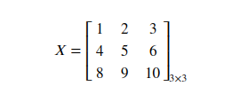
In the above example, since the number of rows (m) = the number of columns (n), X can be termed as a square matrix.
Symmetric Matrix -
A square matrix, X, is termed as symmetric if xᵢⱼ = xⱼᵢ ∀ i and j where i, j denotes the ith row and jth column respectively. In other words, matrix X is symmetric if the transpose of X is equal to matrix X.
Hessian Matrix
The Hessian of a multivariate function f(x₁, x₂, …xₙ) is a way for organizing second-order partial derivatives in the form of a matrix.
Consider a multivariate function f(x₁, x₂, …xₙ) then its Hessian can be defined as follows -
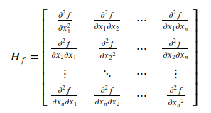
Note that a Hessian matrix by definition is a Square and Symmetric matrix.
Proving / Checking Convexity of a function -
With all the relevant basics covered in previous sections, we are now ready to define checks for determining the convexity of functions.
A function f(x) defined over n variables on an open convex set S can be tested for convexity using the following criteria -
If Xᴴ is the Hessian Matrix of f(x) then -
- f(x) is strictly convex in S if Xᴴ is a Positive Definite Matrix.
- f(x) is convex in S if Xᴴ is a Positive Semi-Definite Matrix.
- f(x) is strictly concave in S if Xᴴ is a Negative Definite Matrix.
- f(x) is concave in S if Xᴴ is a Negative Semi-Definite Matrix.
In the next section, let’s discuss ways to test the definiteness of a matrix.
Positive Definite and Semidefinite Matrices -
You may have seen references about these matrices at multiple places but the definition and ways to prove definitiveness remains elusive to many. Let us start with the textbook definition -
An n × n square matrix, X, is Positive Definite if aXa > 0 ∀ a ∈ ℝⁿ.
Similarly,
An n × n square matrix, X, is Postive Semidefinite if aᵀXa ≥ 0 ∀ a ∈ ℝⁿ.
The same logic can be easily extended to Negative Definite and Negative Semidefinite matrices.
An n × n square matrix, X, is Negative Definite if aᵀXa < 0 ∀ a ∈ ℝⁿ.
And finally,
An n × n square matrix, X, is Negative Semidefinite if aᵀXa ≤ 0 ∀ a ∈ ℝⁿ.
- However, while checking for Matrix Definiteness, validating the condition of every value of `a` is definitely not an option.
- So let us try and break this down even further.
Eigen Values and Eigen Vector -
We know that an eigenvector is a vector whose direction remains unchanged when a linear transformation is applied to it.

Analysis
- It is easy to see that the dot product of a with aᵀ will always be positive.
- Referring back to the definition of positive definite matrix and eq(3), aᵀXa can be greater than zero if and only if λ is greater than zero.
Derived Definition for Matrix Definiteness -
Based on pointers mentioned in the above Analysis we can tweak the formal definitions of Matrix Definiteness as follows -
- A Symmetric Matrix, X, is Positive Definite if λᵢ > 0 ∀ i
- A Symmetric Matrix, X, is Positive Semi-Definite if λᵢ ≥ 0 ∀ i
- A Symmetric Matrix, X, is Negative Definite if λᵢ < 0 ∀ i
- A Symmetric Matrix, X, is Negative Semi-Definite if λᵢ ≤ 0 ∀ i
Alternate Definition for Determining Matrix Definiteness -
- Computing Eigenvalues for large matrices often involves solving linear equations.
- Large Matrices involve solving linear equations in a large number of variables. Hence, it may not always be feasible to solve for Eigen Values.
An Alternate Theorem for Determining Definiteness of Matrices comes to the rescue -
Theorems -
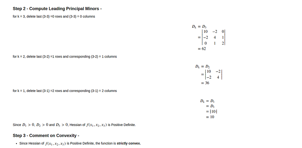
- A Symmetric Matrix, X, is Positive Definite if Dₖ> 0 ∀ k Where Dₖ represents the kth Leading Principal Minor.
- A Symmetric Matrix, X, is Positive Semi-Definite if Dₖ ≥ 0 ∀ k Where Dₖ represents the kth Principal Minor.
- A Symmetric Matrix, X, is Negative Definite if Dₖ< 0 ∀ k Where Dₖ represents the kth Leading Principal Minor.
- A Symmetric Matrix, X, is Negative Semi-Definite if Dₖ≤ 0 ∀ k Where Dₖ represents the kth Principal Minor.
Principal Minors of a Matrix -
- For a Square Matrix, X, a Principal Submatrix of order k is obtained by deleting any (n-k) rows and corresponding (n-k) columns.
- The determinant of such a Principal Submatrix is called the Principal Minor of matrix X.
Leading Principal Minors of a Matrix -
- For a Square Matrix X, a Leading Principal Submatrix of order k is obtained by deleting last (n-k) rows and corresponding (n-k) columns.
- The determinant of such a Leading Principal Submatrix is called the Leading Principal Minor of matrix X.
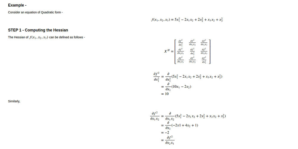
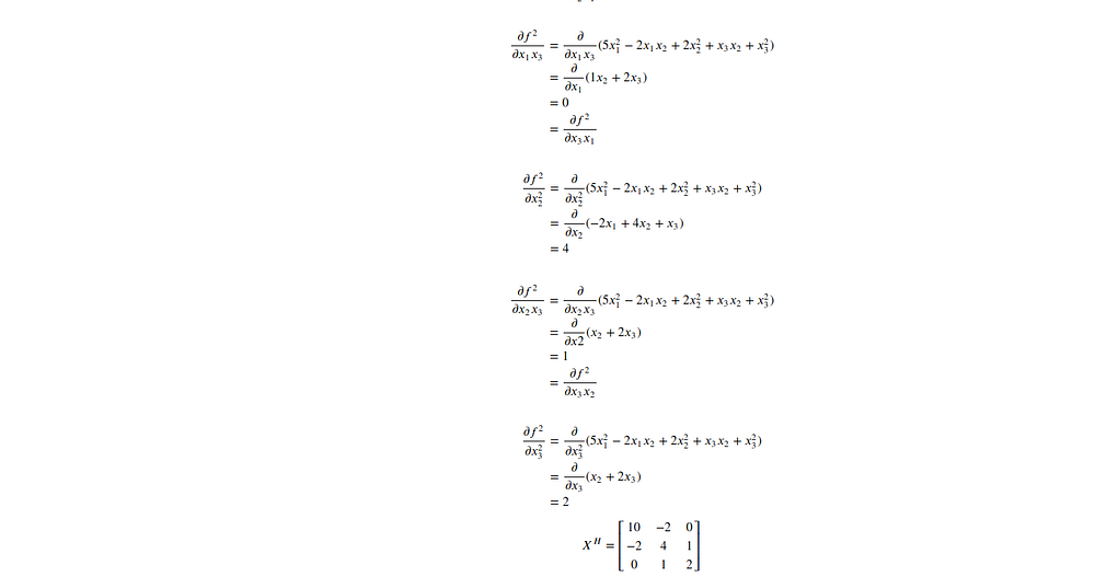
Testing Convexity of a Quadratic Function —
In this section, let's try and apply all the learning from this blog and put it to the test.
Properties of Convex functions -
- Constant functions of the form f(x) = c are both convex and concave.
- f(x) = x is both convex and concave.
- Functions of the form f(x) =xʳ with r ≥ 1 are convex on the Interval 0 < x < ∞
- Functions of the form f(x) = xʳ with 0 < r < 1 are concave on the Interval 0 < x < ∞
- The function f(x) = łog(x) is concave on the interval 0 < x < ∞
- The function f(x) = eˣ is convex everywhere.
- If f(x) is convex, then g(x) = cf(x) is also convex for any positive value of c.
- If f(x) and g(x) are convex then their sum h(x) = f(x) + g(x) is also convex.
Final Comments -
- We have investigated convex functions in depth while studying different ways of proving convexity.
- In the next article, we shall prove the convexity of the MSE loss function used in linear regression.
- Convex functions are easy to minimize thus resulting in their usage across research domains.
- So, the next time you want to plug in a different loss function in place of MSE while training a linear regression model, you might as well check its convexity.
